
Dataset Normalization in Practice
Data Modeling part 8 / Normalization part 4
Data Modeling is an important skill for any data worker to understand. Data Engineers in particular should understand this topic and be able to apply it to their work. Normalization is an important part of Data Modeling and part one of my Normalization series can be found here.
For this post, we will be going over the examples of how normalization works in practice. I will also be reviewing foreign-primary key relationships, as they are the crux of how normalization (increasing normal forms) and denormalization (decreasing normal forms) works.
pt 4: Increasing Normal Forms (this post)
future pt 5: Denormalization in Practice
I recommend you have a fundamental understanding of foreign key relationships and why we would want to normalize a dataset before continuining.
But Why Data Models?
Normalization is a data modeling technique for data workers who want to make sense out of messy datasets. Normalized datasets with tight constraints are also much less likely to create data integrity issues and anomolies. As opposed to standard “cleaning data”, which could relate to the contents e.g. removing white space, normalization is more concerned with the form or structure of the data.
Normalization is represented through “normal forms” which increase from first to third, with a special case not covered here (Boyce-Codd Normal form - BCNM). There are plenty of academic cases increasing past third normal form (3NF), but this starts to work against you in real life for two reasons. The first is that it forces many expensive JOINs across highly partitioned data. The second is that your results may start to look like Star Wars: Foreign Keys Strike Back, without any actual business insights in your dataset results. Putting business needs first, we’ll only go up until 3rd Normal Form.
Decomposition — Increasing normal forms
Both analysts and engineers come across real life messy datasets. This is especially difficult when the columns are all over the place. Decomposition of this dataset, whether ad-hoc or automated, is done to reduce the opportunity for inconsistent and redundant data.
Let us say a dataset looks like
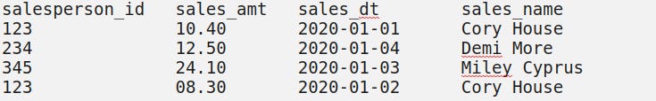
1st Normal Form
Practiced eyes can probably already tell that the id column is not a unique identifier. But before we address primary keys, we need to make sure that every column is atomic and contains indivisible values.
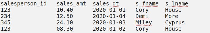
This dataset, with a name split, now meets first normal form requirements because the first and last names have been split into their expected divisible parts.
Please note that as we serve different people from around the world, the first and surname data structure will not always work.
Another common example; splitting up a physical address into its most discrete parts as columns. Quick "Sales Person Address" table example:
sales_id    address
123         '1432 Street St. Boise Idaho 88888'
normalized to first normal form:
sales_id   address_num   street_name   city    State   zip
123        1432          Street St.    Boise   ID      88888
2nd Normal Form
The next two requirements for 2nd normal form is that our dataset meets first normal form requirements and that our dataset has no partial dependencies. What does partial dependency mean? Before we answer that, let’s define candidate key.
Candidate Key : a column or combination of columns that could uniquely represent every single row/piece of data in our dataset. The Candidate Key is often a single column primary key, or unique identifier, but sometimes multiple columns are needed.

For example, in our first table we would need both the salesperson_id and the sales_dt (assuming it is also storing time in hhmmss hours-minutes-seconds) to be able to extract specific rows from our dataset.

Having only one filtering condition, a salesperson_id, may return duplicate tuples or rows. By definition, this doesn't meet our insights unique identification requirements.
Do we have a single unique identifying (ID, Primary Key, or Code of some kind) column that will give us all relevant information from our database?
Going back to our first normal form dataset (before):
We have a candidate key of `salesperson_id` and `sales_dt` (assuming the time is also being recorded here). But `sales_name` is entirely a subset of our `salesperson_id` column, which is not a candidate key.
Whereas in first normal form, you’re more likely to split up columns, in second, you’re more likely to split up tables. Second normal form dataset (after):
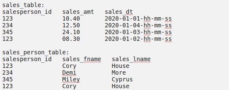
Primary and Foreign Key talk:
Here, the combination of `salesperson_id` and `sales_dt` is the candidate key or primary key of our `sales_table`. What is also true is that `salesperson_id` is the foreign key in our `sales_table` which may allow to to join with the `salesperson_id`, which is the primary key for `sales_person_table`.
This is particularly useful when dealing with relational databases, trying to minimize duplicate data and potential for data integrity issues down the line. We have better structured our dataset, while still the keeping wholeness and integrity of it.
Warning: As a database goes through more normalization, you can imagine the number of JOINs required in queries also goes up. Keep these trade-offs in mind.
3rd Normal Form
A dataset, table, or relation is in 3rd Normal Form (3NF) when 2NF requirements are met and there are no transitive dependencies; columns that have a chaining identification within the same table.
Practically; third normal form says that all columns in your tables should have a single unique identifier in that same table. Primary Key Column A may point to Column B, but the same table should not contain a Column C which our Column B points to. All unique identifications should be umbrella’d under the original Primary Key/Column A for each relation or table.
Our 2NF dataset already meets this requirement, but it is not hard to imagine more columns being appended to create a transitive dependency.
For example; adding three columns `sales_item_id`, `sales_item_line` and `sales_item_name` to our `sales_table` would require us to create a new table called `sales_item` with primary key `sales_item_id`.

The reason is that `sales_item_name` and `sales_item_line` both depend on `sales_item_id`, which depends on our original combination primary key of `sales_dt` and `salesperson_id`.

This is all assuming a salesperson can only sell one item per transaction.
Having a chaining dependency breaks our 3NF requirement. Instead of listing out every item name and product line for every transaction in `sales_table`, we can store our inventory uniquely in a smaller table. Adherence to 3NF would further split out hypothetical dataset into three tables: sales transactions, persons, and items.
Finale
This decomposition technique is useful for both analysts and engineers because it is common to have to apply it to both ad-hoc and repeatable/automated processes. In the next post, we will go over real life examples of denormalization and how I’ve seen it applied at high business need environments.
Curated Content
Bi-directional webhooks and APIs to familiarize yourself with modern dataflows
Data Architecture as it relates to your SQL and JSON data
For non traditional (small schools, small companies, career pivoters) job candidates:
 Wes Kao@wes_kaoIf you are a non-traditional job candidate... Without proper framing it's usually a bad thing. You're risky on paper. But w/proper framing you can be in a category of one. Proactively frame your experience. Why you are everything they need & didn't even know they needed4:41 PM · Feb 15, 202116 Reposts · 111 Likes
About the Author and Newsletter
I am a small tech business owner of a data infrastructure consultancy shop, Ocelot Data. Ocelot Data is the data infrastructure services shop. Contact us to get the data that you need to execute on your operations and marketing goals. We have taken on consultancy projects at Stripe, Capital One, and Redmonk.
At Modern Data Infrastructure, I democratize the knowledge it takes to understand an open-source, transparent, and reproducible Data Infrastructure. In my spare time, I collect Lenca pottery, walk my dog, and listen to music.
More at; What is Modern Data Infrastructure.